Overview of Recommender Algorithms – Part 2

This is the second in a multi-part post. In the first post, we introduced the main types of recommender algorithms by providing a cheatsheet for them. In this post, we’ll describe collaborative filtering algorithms in more detail and discuss their pros and cons in order to give a deeper understanding for how they work.

Collaborative filtering (CF) algorithms look for patterns in user activity to produce user specific recommendations. They depend on having user usage data in a system, for example user ratings on books they have read indicating how much they liked them. The key idea is that the rating of a user for a new item is likely to be similar to that of another user, if both users have rated other items in similar way. It is worth noting that they do not depend on having any additional information about the items (e.g. description, metadata, etc) or the users (e.g. interests, demographic data, etc) in order to generate recommendations. Collaborative filtering approaches can be divided into two categories: neighbourhood and model-based methods. In neighbourhood methods (aka memory-based CF), the user-item ratings are directly used to predict ratings for new items. In contrast, model-based approaches use the ratings to learn a predictive model based on which predictions on new items are made. The general idea is to model the user-item interactions using machine learning algorithms which find patterns in the data.

Neighbourhood-based CF methods focus on the relationship between items (item-based CF), or alternatively, between users (user-based CF).

• User-Based CF finds users who have similar appreciation for items as you and recommends new items based on what they like.
• Item-based CF recommends items that are similar to the ones the user likes, where similarity is based on item co-occurrences (e.g. users who bought x, also bought y).

First, we’ll look at user-based collaborative filtering with a worked example before doing the same for the item-based version.

Say that we have some users who have expressed preferences for a range of books.  The more that they like the book, the higher a rating they give it, from a scale of one to five.  We can represent their preferences in a matrix, where the rows contain the users and the columns the books (Figure 1).

Figure 1: User preferences for books.  All preferences are on a scale of 1-5, 5 being the most liked.  The first user (row 1) has a preference for the first book (column 1) given by a rating of 4.  Where a cell is empty, the user has not give a preference for the book.

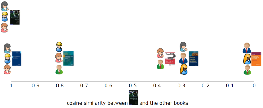
In user-based collaborative filtering, the first thing that we want to do is to calculate how similar users are to one another based on their preferences for the books.  Let’s consider this from the perspective of a single user, who appears in the first row in Figure 1.  To do this, it’s common to represent every user as a vector (or array) that contains the user preferences for items.  It’s quite straight-forward to compare users with one another using a variety of similarity metrics.  In this example, we’re going to use cosine similarity.  When we take the first user and compare them to the five other users, we can see how similar the first user is to the rest of them (Figure 2).  As with most similarity metrics, the higher the similarity between vectors, the more similar they are to one another.  In this case, the first user is quite similar to two users, as they share two books in common, less similar to two other users, who share just one book in common and not at all similar to the last user with whom they share no books in common.

Figure 2: The similarity between the first user and the rest of the users.  This can be plotted in a single dimension using the cosine similarity between users.

More generally, we can calculate how similar each user is to all users and represent them in a similarity matrix (Figure 3).  This is a symmetric matrix which, as an aside, means that it has some useful properties for performing mathematical functions on it.  The background colour of the cells indicates how similar the users are to one another, the deeper red they are the more similar.

Figure 3: Similarity matrix between users.  Each user similarity is based on the cosine similarity between the books that the users read.

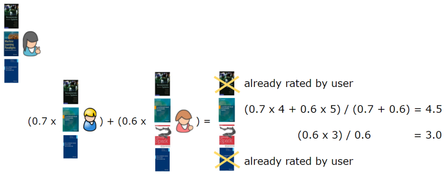
Now we’re ready to generate recommendations for users, using user-based collaborative filtering.  In general, for a given user, this means finding the users who are most similar to them, and recommending the items that these similar users appreciate, weighting them by how similar the users are.  Let’s take the first user and generate some recommendations for them.  First, we find the top n users who are most similar to the first user, remove books that the user has already given preferences for, weight the books that the most similar users are reading, and sum them together.  In this case, we’ll take n = 2, that is the two users who are most similar to the first user, in order to generate the recommendations.  These two users are users 2 and 3 (Figure 4).  Since, the first user already has rated books 1 and 5, the recommendations generated are books 3 (score of 4.5) and 4 (score of 3).

Figure 4: Generating recommendations for a user.  We take the books that they two most similar users are reading, weight them, and recommend the books that are not yet rated by the user.

So now that we have a better feeling for user user-based collaborative filtering, let’s look through an example of item-based collaborative filtering. Again, we start with the same set of users who have expressed preferences for books (Figure 1).

In item-based collaborative filtering, similar to user-based, the first thing that we want to do is to calculate a similarity matrix.  This time round, however, we want to look at similarities with respect to items rather than users.  Similarly, we show how similar a book is to other books if we were to represent books as vectors (or arrays) of users who appreciate them and to compare them with the cosine similarity function.  The first book, in column one, is most similar to the fifth book, in column five, as it is appreciated roughly the same by the same set of users (Figure 5).  The third most similar book is appreciated by two of the same users, the fourth and second books only have one user in common while the last book is not considered to be similar at all as it has no users in common.

Figure 5: Comparison of the first book to the rest of them.  Books are represented by the users who have rated them.  Comparisons are made using the cosine similarity metric (0-1).  The higher the similar, the more similar the two books.

More fully, we can show how similar all books are to one another in a similarity matrix (Figure 6).  Again, the background colour of the call shows how similar two books are to one another, the darker the red, the more similar they are.

Figure 6: Similarity matrix for books.

Now that we know how similar the books are to one another, we can generate recommendations for users.  In the item-based approach, we take the items that a user has previously rated, and recommend items that are most similar to them.  In our example, the first user would be recommended the third book followed by the sixth book (Figure 7).  Again, we only take the top two most similar books to the books that the user has previously rated.

Figure 7: Generating recommendations for a user.  We take the books that they have rated, find the two most similar books to each of them, weigh them and recommend the books that the user has not yet rated.

Given that the descriptions of user-based and item-based collaborative filtering sound very similar to one another, it’s interesting to note that they can generate different results.  Even in the toy example that we give here, the two approaches generate different recommendations for the same user even though the input is the same to both.  It’s worth considering both of these forms of collaborative filtering when you’re building your recommender.  Although when describing them to non-experts they can sound very similar, in practice they can give quite different results with qualitatively different experience for the user.

Neighbourhood methods enjoy considerable popularity due to their simplicity and efficiency, and their ability to produce accurate and personalised recommendations. However, they also have some scalability limitations as they require a similarity computation (between users or items) that grows with both the number of users and the number of items. In the worst case this computation can be O(m*n), but in practice the situation is slightly better with O(m+n), partly due to exploiting the sparsity of the data. While sparsity helps with scalability, it also presents a challenge for neighbourhood-based methods because we only have user ratings for small percentage of the large number of items. For example, at Mendeley we have millions of articles and a user may have read a few hundred of these articles. The probability that two users who have each read 100 articles have an article in common (in a catalogue of 50 million articles) is 0.0002.

Model-based CF approaches can help overcome some of the limitations of neighbourhood-based methods. Unlike neighbourhood methods which use the user-item ratings directly to predict ratings for new items, model-based approaches use the ratings to learn a predictive model based on which predictions on new items are made. The general idea is to model the user-item interactions using machine learning algorithms which find patterns in the data. In general, model-based CF are considered more advanced algorithms for building CF recommenders. There are a number of different algorithms that can be used for building the models based on which to make predictions, for example, bayesian networks, clustering, classification, regression, matrix factorisation, restricted boltzmann machines, etc. Some of these techniques played a key role in the final solutions for winning the Netflix Prize. Netflix ran a competition from 2006 to 2009 offering $1mil grand prize to the team that can generate recommendations that were 10% more accurate than their recommender system at the time. The winning solution was an ensemble (i.e. mixture) of over 100 different algorithm models of which matrix factorisation and restricted boltzmann machines were adopted in production by Netflix.

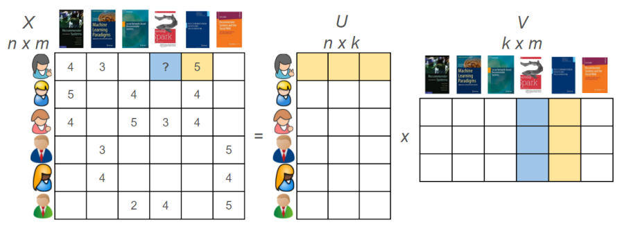
Matrix factorisation (e.g. singular value decomposition, SVD++) transforms both items and users to the same latent space which represents the underlying interactions between users and items (Figure 8). The intuition behind matrix factorisation is that the latent features represent how users rate items. Given the latent representations of the users and the items, we can then make predictions of how much the users will like items they have not yet rated.

Figure 8: Representation of matrix factorisation.  A user preference matrix can be decomposed into a user-topic matrix multiplied by a topic-item matrix.

In Table 1, we outlined the key pros and cons of both neighbourhood and model-based collaborative filtering approaches. Since they depend only on having usage data of the users, CF approaches require minimal knowledge engineering efforts to produce good enough results, however, they also have limitations. For example, CF tends to recommend popular items, making it hard to recommend items to someone with unique tastes (i.e. interested in items which may not get so much usage data). This is known as the popularity bias and it is usually addressed with content-based filtering methods. An even more important limitation of CF methods is what we call “the cold start problem”, where the system is not able to give recommendations for users who have no (or very little) usage activity, aka new user problem, or recommend new items for which there is no (or very little) usage activity, aka new item problem. The new user “cold start problem” can be addressed via popularity and hybrid approaches, whereas new item problem can be addressed using content-based filtering or multi-armed bandits (i.e. explore-exploit). We’ll discuss some of these methods in the next post.

In this post we covered three basic implementations of collaborative filtering.  The differences between item-based, user-based and matrix factorisation are quite subtle and it’s often tricky to explain them succinctly.  Understanding the differences between them will help you to choose the most appropriate algorithm for your recommender.  In the next post we’ll continue to look at popular algorithms for recommenders in more depth.